New to
climate information?

This is a learning zone where you can learn more about climate information. It provies basic knowledge about climate models, emission scenarios and much more.  

How to calculate the impacts of climate change?

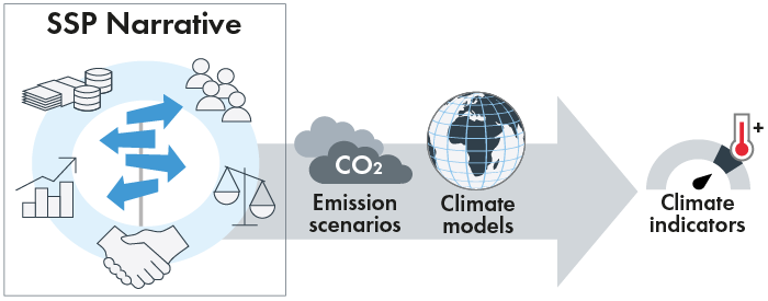
The climate indicators provided at climateinformation.org are the end result of a long chain of model simulations and statistical calculations. Here we first provide a general overview of how to estimate local changes in climate indicators with the necessary steps for an impact assessment. After the overview we provide more in-depth information about models and methods along the chain.

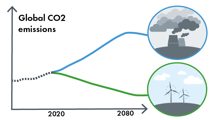
From greenhouse gas emissions to future climate trends

A starting point is the emissions scenarios. What would you like to look at? Business-as-usual or a moderate path? Scenarios for the evolution of greenhouse gas emissions are provided by Representative Concentration Pathways (RCPs) or Shared Socioeconomic Pathways (SSPs).

Emission scenarios depending on future development.

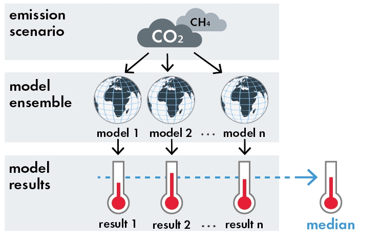
Global Climate Models (GCMs) are then applied to calculate projections of how the emissions affect climate. The various GCMs differ in their sensitivity to the greenhouse gas forcing, and also in how they simulate different processes in the Earth’s climate; each having their own strengths and weaknesses. An ensemble of models has proven more reliable, as the uncertainties stemming from the different models to some degree cancel each other. Ensemble statistics, e.g. the median result from of a number of models, are therefore generally considered more reliable than using a single model projection.

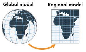
GCMs have a typical horizontal resolution of several hundred kilometers, and since e.g. most hydrological processes occur at much smaller scales, a further downscaling of the GCM information is useful . This is performed by Regional Climate Models (RCMs), which nest into the GCM and provide finer scale information of 50 km or less. CMIP(Coupled Model Intercomparison Project) and CORDEX (Coordinated Regional climate Downscaling EXperiment) are two global collaboration programs under WCRP (the World Climate Research Program) of WMO (World Meteorological Organization) that coordinate GCM and RCM ensembles respectively.

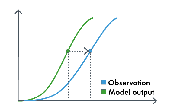
Hydrological and other impact modelling applications are sensitive to climate model bias. Bias is a systematic deviation from observed statistics, e.g. consistently too wet or too warm climate in a certain region of the world. It is common practice to apply bias adjustment, a statistical method that removes various errors from the climate model output so that they become more similar to observations (local gridded or station data) or reanalysis.

Climate and water indicators are produced, at the end of the computation chain, to show how the climate changes between different time periods and for a given emission scenario. Since climate is an average of the weather over a long period of time, indicators are often produced as an average over thirty years.

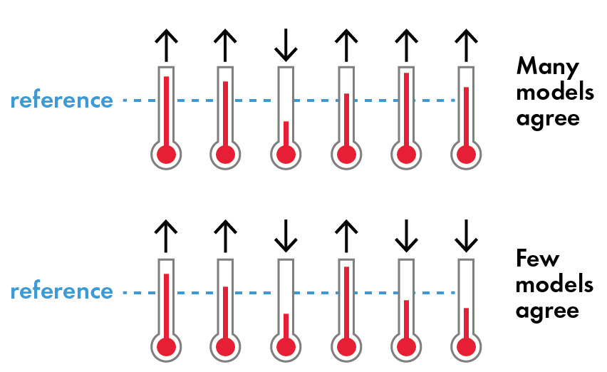
Each model step in the production chain includes uncertainties, with the main uncertainty within each emission scenario arising from the climate models. Therefore, an ensemble of projections (multiple RCMs and/or GCMs) is used to account for the spread of possible climate impacts in the future. The uncertainties inform about the reliability of the climate projection, e.g. if all models agree on the sign of the change, and how well they agree on the magnitude of the change. The exact future still remains unknown but the indicators show tendencies and future risks generated by climate change.

Agreement on sign of change compared to reference period.

Models and Methods

In this section you can learn about the models and methods used in production of climate indicators. This is a basis for understanding the possible choices in the tools available at climateinformation.org.

What is a climate model?

Climate models are our main tools for calculating the future and historic climate. Scientists often use climate models to study how the climate may change when the composition of the atmosphere changes with, for example, changed levels of greenhouse gases and aerosols.

The climate models are three-dimensional mathematical descriptions of the climate system: the atmosphere, land surface, oceans, lakes and ice. In a climate model, the atmosphere is divided into so-called grids along the earth’s surface that extend up into the air, as visualized in the figure.

Climate model

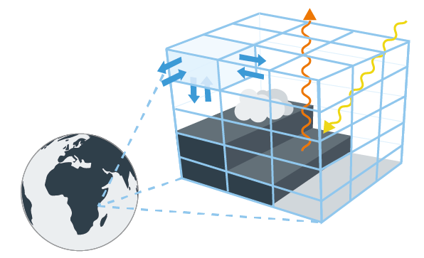
The movements of the atmosphere and the preservation of energy, water and mass follow well-known physical laws that can be described by mathematical formulas. For each grid various processes are calculated, such as heat, wind, generation of clouds and precipitation. A global climate model (GCM) describes many processes both in the atmosphere, ocean, land and cryosphere such as glaciers and ice-caps. A regional model relies on input from the global model and can focus on local processes.

It requires a lot of computer power to run a climate model, and even though the computing capacity is constantly increasing, calculations in the global climate models are still made with a rather sparse grid of several hundred kilometers. This means that the level of detail on a local or regional scale is low in the global model. However, if you want to study a smaller part of the Earth in more detail, you can use so called regional climate models (RCM). In a regional model, the grid is positioned over a smaller area, which means that you can get a denser grid (and more detail, e.g. 50 kilometers) with lower computing power. What happens outside the calculation area in a regional climate model is governed by the results of a global climate model. In this way changes that take place outside the regional model area are considered. This way of using the results from a global model in a regional model is called regional downscaling.

What is the difference between climate and weather?

Weather is what we experience every day, whereas climate is the long-term statistics of weather. It describes for example the mean temperature for a particular place and time-of-year. Weather has a chaotic behavior and is generally only predictable for up to ten days. Climate is governed by more slowly varying processes, and changes can be described when some of these processes change, such as the composition of greenhouse gases.

What is a model ensemble?

Across the globe there are many different climate models being developed. The all describe the main well-known physical laws that govern the atmospheric and oceanic motions, but there are processes that are less well known that can only be estimated with different assumptions. This is done in different ways and at varying complexity by the different models. This means that all climate models will give somewhat different results, and still it is not possible to state which one is more correct. The size of these differences can be large or small depending on model, region, season, variable etc. Some models may perform well for a specific region/season/variable and some worse for other. So even though the climate models are advanced they are not a perfect description of the climate system, but the differences between the climate models carry important and useful information that describes the uncertainty in our knowledge about future climate.. When exploring climate change, one should therefore use several different models, i.e. model ensembles. The spread in the results of the ensemble can be significant, partly because models describe climatological processes in different ways. The advantage of model ensembles is that if the same response is seen in several models the result is considered to be certain. If the responses are different in different models the result is considered to be less certain. Scientist collaborate under different projects and programs. Two important and global programs are: Coupled Model Inter-comparison Project (CMIP) and Coordinated Regional Climate Downscaling experiment (CORDEX).

What is CMIP?

Coupled Model Inter-comparison Project is the standard experimental protocol for studying the output of coupled atmosphere-ocean global climate models . CMIP provides a community-based infrastructure that supports climate model diagnosis, validation, inter-comparison, documentation and data access. This framework enables a diverse community of scientists to analyze the global models in a systematic fashion, a process which helps make models better. The international climate modelling community has participated in this project since it began in 1995. CMIP has been going through several phases, from CMIP1 to CMIP3, then synchronized with the IPCC assessment reports’ numbering with CMIP5 and CMIP6. Each time with some changes to the modelling protocols and standards, e.g. the emission scenarios (RCPs in CMIP5 and SSPs in CMIP6).
Figure? Logo?

What is CORDEX?

Coordinated Regional Climate Downscaling experiment (CORDEX) is responsible to advance and coordinate the science and application of regional climate downscaling models through global partnerships. The project office is hosted by SMHI since 2009. Both CMIP and CORDEX are international collaborations between scientific institutions. They are also diagnostic model inter-comparison projects (model development) for different regions across the world. The programs also help evaluate how realistic the models are in simulating the recent past as well as provide projections of future climate change. CMIP6, CMIP5 and CORDEX are endorsed by the World Climate Research Program (WCRP). Information from CMIP5 and CORDEX experiments are summarized in the Intergovernmental Panel on Climate Change (IPCC) reports, starting from the IPCC Fifth Assessment Report (IPCC AR5), and CMIP6 are introduced in the assessment report as of the IPCC Sixth Assessment Report (IPCC AR6). CORDEX experiments are frequently used in regional assessment reports. The CORDEX regions sometimes differ regarding their spatial resolution.

Figure? Logo?

What is an emission scenarios?

Emission scenarios describe possible anthropogenic emissions of greenhouse gases, based on assumptions about the future development of the world’s economy, population growth, globalization, transition to environmentally friendly technology and more. All this affects the level of greenhouse gas emissions, which in turn affects the greenhouse effect. One way of measuring how the greenhouse effect will change in the future is to estimate radiative forcing, which is measured in power per square meter (W/m2). More greenhouse gases in the atmosphere lead to a higher additional radiative forcing. Such scenarios are called Representative Concentration Pathways (RCP), and are in CMIP6 accompanied by further information about e.g. land-use changes in the Shared Socio-economic Pathways (SSP).

What is RCP?

Every RCP-scenario (Representative Concentration Pathways) represents a future with different levels of emissions (and radiative forcing). On this platform three scenarios are used: 2.6, 4.5 and 8.5. Read more what they mean in the article “What do different RCPs mean?”. Apart from RCP scenarios, Shared Socio-economic Pathways (SSPs) are also used in the climate models. These pathways are a separate complementary effort to look at factors such as population, education, economic growth, urbanization and technological development. Theoretically, each SSP can be used alongside the RCPs as long as it goes with the narrative (that will be explained below). While the RCP are used as input to evaluate the level of global warming in the future considering the levels of emissions, the SSPs look at the possibilities of emission reduction. SSPs can be combined with climate impact scenarios (as RCP scenarios) as well as sets of policy assumptions to study for example the interactions between climate change, related climate impacts, vulnerability to these and possible actions. But what are Shared Socio-economic Pathways?

What is SSP?

The SSP-scenarios (Shared Socio-economic Pathways) are five scenarios that describes different socio-economic developments used in climate models. The SSPs has been introduced because the climate is changing due to the emission of carbon dioxide, other greenhouse gases and the change of land use . These factors such as emissions of carbon dioxide, other greenhouse gases and the change of land use are crucial to describe the evolution of the future anthropogenic climate forcings and, and therefore the climate scenarios need to take these factors into account. The SSPs differ in terms of, among other things, population development, equality, energy use and global carbon dioxide emissions. In all SSPs, the global economy is growing. Read more about the characteristics of the SSPs in the article “What is SSPs? and What is the difference between SSPs and RCPs? ”. 

SSP narratives describing alternative socio-economic developments

None of the SSPs are more likely than the other but the world can develop in several different ways depending on decisions in a number of different areas, where different paths are possible. All SSPs pose different major challenges for emission reductions and adaptation. However, no actual climate policy is included in these scenarios. Although climate policies can be explored in studies based on the conditions provided by the scenarios, for example to achieve a certain emission reduction.

What is a climate scenario?

A climate scenario is a description of a possible future evolution of the climate, as calculated by a climate model based on an emission scenario. Climate scenarios are several possible climate developments that require a long chain of assumptions and calculations. The description of the scenario can be in the form of, for example, a map, a diagram or a table. The values can be absolute numbers, differences, or related to a value like for example time. The standard period to measure climate change is 1961-1990. However, for climateinformation.org the focus is on describing changes from the latest experienced climate period, which is why the later WMO standard reference periods are used. For the CMIP5 (RCP) information in climateinformation.org, a reference period 1981-2010 is used, but for the calculation of the CMIP6 data, the latest period 1991-2020 is used. Therefore, the climate change signals may appear weaker when comparing the CMIP5 and CMIP6 data in the portal.

What is bias adjustment?

The complex climate system, with many interdependent processes that are not always fully known or described in the climate model, inevitably leads to the climate model producing systematic deviations from observed values. These systematic deviations are called model bias. The bias can be of different magnitude for different variables and for different regions of the world. Most often, these deviations do not pose a problem for calculating climate indicators where the focus is on differences between a historical and a future scenario. However, some indicators are based on absolute limits, such as the number of days with frost, tropical nights, or precipitation above a certain level. A bias in the climate model can affect these indicators so that their interpretation is misleading. To remedy such issues, the variables are bias adjusted using a scientific developed method based on defining a mapping of the range of model values to an observed range of values. The method used here is called quantile mapping, and two different versions of this technique are used depending on the production time of the indicators. The CMIP5 (those using RCP emission scenarios) models are bias adjusted using the Distribution Based Scaling (Yang et al., 2010), and the CMIP6 uses the newly developed method MIdAS (Berg et al., 2022).

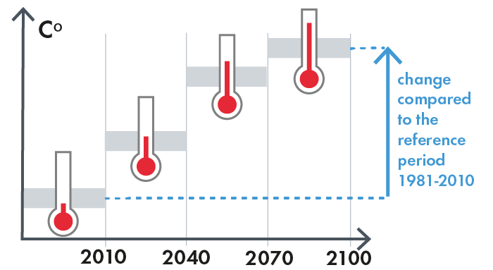
What is a climate indicator?

A climate indicator presents a parameter that describes the climate for a given longer time period. It can for example be average temperature, global radiation and days with snow cover, or using hydrological impact models, for example the annual river discharge. Many of the climate indicators are presented as deviations from a reference period to describe how climate is changing. Here, the reference periods 1981-2010 is used for CMIP5 based indicators, and 1991-2020 for CMIP6 based indicators.


What are water impacts?

climateinformation.org shows climate change effects on hydrological variables along with the meteorological indicators. Climate change is affecting the hydrological cycle and this is calculated with the hydrological impact model World Wide HYPE (WWH). The HYPE model calculates the discharge in rivers, surface runoff and other hydrological parameters based on mathematical representations of storage and flow processes in and on the ground, and in lakes and streams. The WWH model divides the world in river catchments based on how water flows through the landscape. Water and energy balance equations, as well as routing of water through rivers is described, and lakes and human regulation of flows are included in the model. Bias adjusted climate model data of daily mean precipitation, and daily mean, minimum and maximum temperature is used as input to simulate the hydrological impacts with WWH. Ev. Länkar till mer detaljerade sidor

Robustness and uncertainties

Uncertainties in the type of results presented in the analyses are affected by the choice of emission scenarios, global climate model, regional climate model, hydrological model and natural variability. These uncertainties lead to a spread in the results for a given climate indicator. The ensemble mean (as presented in the maps) is the most robust statistic from the models, as shown in numerous scientific studies. However, the spread in the results is an important information that can be used to guide the interpretation of future climate change. The spread in the results can inform about how robust the changes are. For example, do all or most models project the same sign of the change? Sometimes the uncertainty (spread) is large, but still all models consistently show and increase for the indicator. This is a robust result that points to an increase, although with uncertainty of the magnitude of the change. Sometimes there is a mix of about half of the models showing an increase, and the other half showing a decrease. The change is not robust in this case. Ev. Länkar till mer detaljerade sidor